44 excel pivot table labels

Changing Blank Row Labels - Excel Pivot Tables You can manually change the (blank) labels in the Row or Column Labels areas by typing over them in the pivot table. You can type any text to replace the (Blank) entry, but you can't clear the cell and leave it empty: Select one of the Row or Column Labels that contains the text (blank). Type N/A in the cell, and then press the Enter key. Use column labels from an Excel table as the rows in a Pivot Table Close the dialog and keep the changes. Excel should place the unpivoted data into a new worksheet, looking something like this: Now the final step is to create a pivot table using this unpivoted data. Here is a screenshot of my pivot table setup: Note that Attribute (e.g. Malaria, Tuberculosis) is placed above the Year. This lets us open or ...

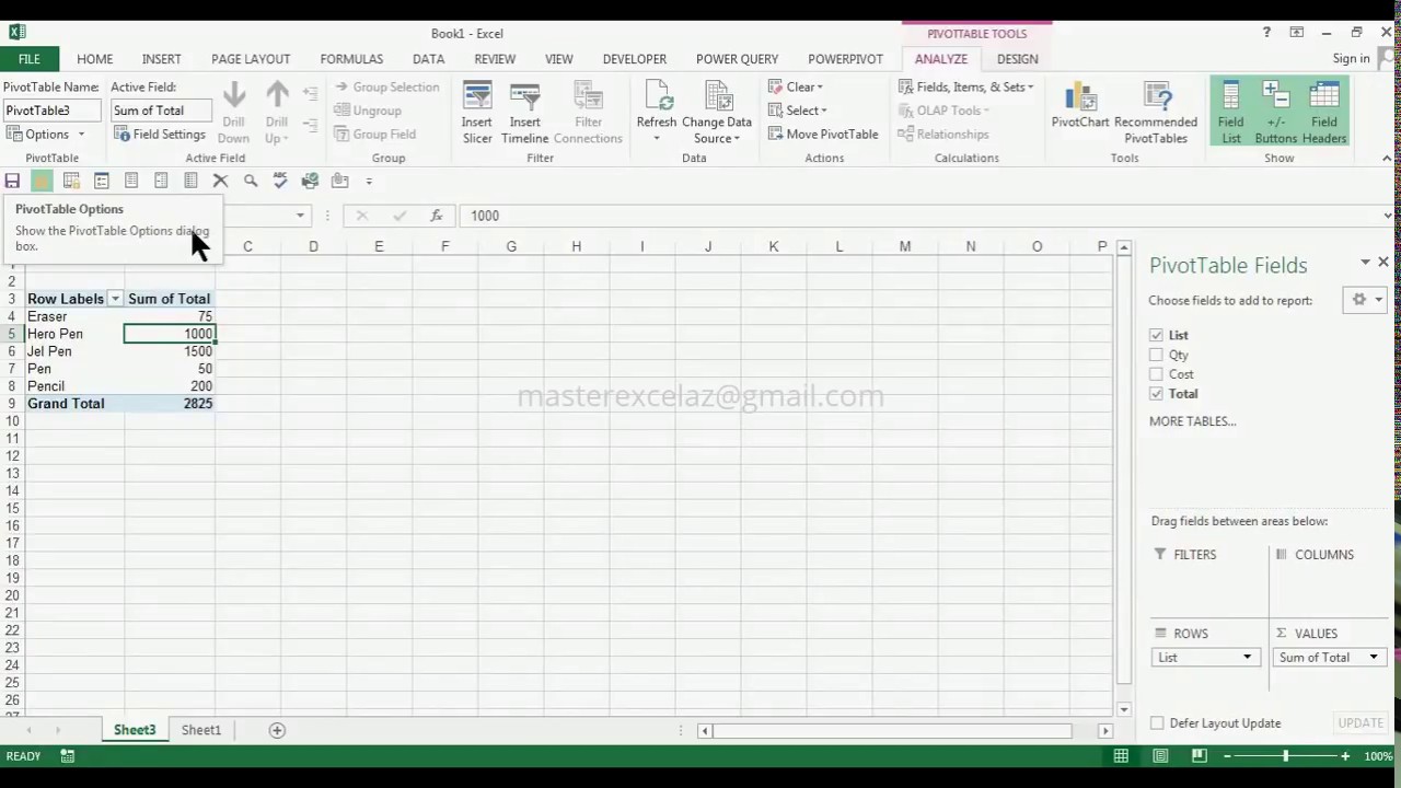
How to Move Excel Pivot Table Labels Quick Tricks To move a pivot table label to a different position in the list, you can use commands in the right-click menu: Right-click on the label that you want to move Click the Move command Click one of the Move subcommands, such as Move [item name] Up The existing labels shift down, and the moved label takes its new position. Type Over Another Label

Excel pivot table labels

Pivot table row labels in separate columns • AuditExcel.co.za Our preference is rather that the pivot tables are shown in tabular form (all columns separated and next to each other). You can do this by changing the report format. So when you click in the Pivot Table and click on the DESIGN tab one of the options is the Report Layout. Click on this and change it to Tabular form. How to Customize Your Excel Pivot Chart Data Labels - dummies The Data Labels command on the Design tab's Add Chart Element menu in Excel allows you to label data markers with values from your pivot table. When you click the command button, Excel displays a menu with commands corresponding to locations for the data labels: None, Center, Left, Right, Above, and Below. How to add column labels in pivot table [SOLVED] Steps:-. Click any date in the Column Lables. Click Pivot table options tab on the Ribbon. In the Options Table, Click Group Field option. Click Months then click Ok. Thats it. check the attached file:-. Attached Files. PIVOT.xlsx‎ (30.3 KB, 6 views) Download.

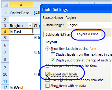
Excel pivot table labels. Repeat item labels in a PivotTable - support.microsoft.com Right-click the row or column label you want to repeat, and click Field Settings. Click the Layout & Print tab, and check the Repeat item labels box. Make sure Show item labels in tabular form is selected. Notes: When you edit any of the repeated labels, the changes you make are applied to all other cells with the same label. Excel 2016 Pivot table Row and Column Labels - Microsoft Community In Excel 2016 I've found when I create a pivot table it unhelpfully shows 'Row Labels' and 'Column Labels' instead of my field names, although in the top left cell it says 'Count of' and then inserts the correct field name. Years ago when I last used Excel it automatically put the field names in all three heading cells. Pivot Table column label from horizontal to vertical Pivot Table column label from horizontal to vertical After pivot table and with grouping, some column labels have been showed but the caption is on the top. What i want is put the column header at the left of the row as vertical red text show as below. However, i cannot do this, it said "We cant change this part of pivot table". Remove row labels from pivot table • AuditExcel.co.za Click on the Pivot table. Click on the Design tab. Click on the report layout button. Choose either the Outline Format or the Tabular format. If you like the Compact Form but want to remove 'row labels' from the Pivot Table you can also achieve it by. Clicking on the Pivot Table. Clicking on the Analyse tab.

Change the pivot table "Row Labels" text | MrExcel Message Board Feb 4, 2021. #3. mart37 said: Click on the cell and typ the text. Click to expand... Thanks mart37. So simple! I was looking for a way to change it on the ribbons & settings. Typical Excel - things you think are difficult are easy, and things that should be easy are difficult! Pivot Table "Row Labels" Header Frustration - Microsoft Tech Community Small and Medium Business. Public Sector. Internet of Things (IoT) Azure Partner Community. Expand your Azure partner-to-partner network. Microsoft Tech Talks. Bringing IT Pros together through In-Person & Virtual events. MVP Award Program. Find out more about the Microsoft MVP Award Program. Remove PivotTable Duplicate Row Labels [SOLVED] Re: Remove PivotTable Duplicate Row Labels. Sometimes when the cells are stored in different formats within the same column in the raw data, they get duplicated. Also, if there is space/s at the beginning or at the end of these fields, when you filter them out they look the same, however, when you plot a Pivot Table, they appear as separate ... Pivot table row labels side by side - Excel Tutorials You can copy the following table and paste it into your worksheet as Match Destination Formatting. Now, let's create a pivot table ( Insert >> Tables >> Pivot Table) and check all the values in Pivot Table Fields. Fields should look like this. Right-click inside a pivot table and choose PivotTable Options…. Check data as shown on the image below.

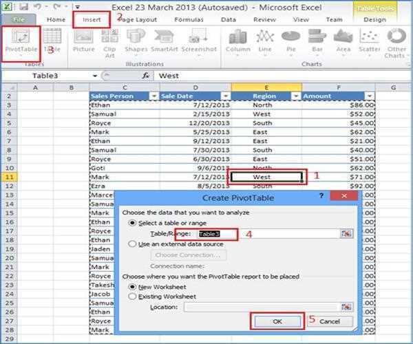
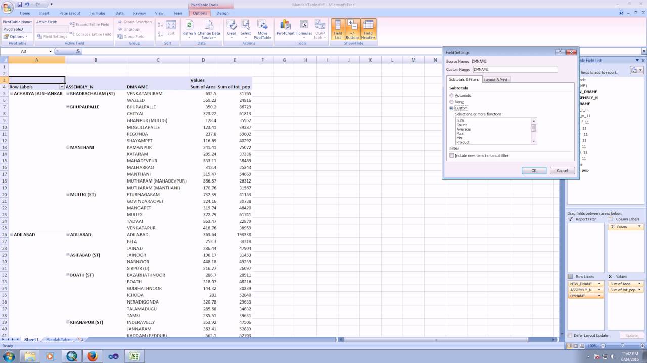
Automatic Row And Column Pivot Table Labels - How To Excel At Excel Select the data set you want to use for your table The first thing to do is put your cursor somewhere in your data list Select the Insert Tab Hit Pivot Table icon Next select Pivot Table option Select a table or range option Select to put your Table on a New Worksheet or on the current one, for this tutorial select the first option Click Ok How to rename group or row labels in Excel PivotTable? 1. Click at the PivotTable, then click Analyze tab and go to the Active Field textbox. 2. Now in the Active Field textbox, the active field name is displayed, you can change it in the textbox. You can change other Row Labels name by clicking the relative fields in the PivotTable, then rename it in the Active Field textbox. Excel: How to Sort Pivot Table by Date - Statology Before creating a pivot table for this data, click on one of the cells in the Date column and make sure that Excel recognizes the cell as a Date format: Next, we can highlight the cell range A1:B10, then click the Insert tab along the top ribbon, then click PivotTable, and insert the following pivot table to summarize the total sales for each ... Design the layout and format of a PivotTable In the PivotTable Options dialog box, click the Layout & Format tab, and then under Layout, select or clear the Merge and center cells with labels check box. Note: You cannot use the Merge Cells check box under the Alignment tab in a PivotTable. Change the display of blank cells, blank lines, and errors

Pivot Table in Excel

How to Use Excel Pivot Table Label Filters In an Excel pivot table, you might want to hide one or more of the items in a Row field or Column field. To do that, you could click the drop down arrow for the Row or Column Labels, then remove the check mark for items you want to remove. For example, to hide the data for 7-Feb-10, you'd click on the check mark to remove it.

Use excel pivot table layout to add label to entry - Stack Overflow

How to unbold Pivot Table row labels | MrExcel Message Board Under the binocular tab, called FIND AND SELECT, select SELECT OBJECTS. This should place a thin blue line around that and all other subtotals at the same level. Make the changes you want (such as unbolding). P pschommer New Member Joined Nov 18, 2006 Messages 10 Dec 10, 2010 #3 After turning on 'Select Objects', the Font options are grayed out.

How to group (two-level) axis labels in a chart in Excel?

Repeat All Item Labels In An Excel Pivot Table | MyExcelOnline DOWNLOAD EXCEL WORKBOOK. STEP 1: Click in the Pivot Table and choose PivotTable Tools > Options (Excel 2010) or Design (Excel 2013 & 2016) > Report Layouts > Show in Outline/Tabular Form STEP 2: Now to fill in the empty cells in the Row Labels you need to select PivotTable Tools > Options (Excel 2010) or Design (Excel 2013 & 2016) > Report Layouts > Repeat All Item Labels

Hide Excel Pivot Table Buttons and Labels – Excel Pivot Tables

Change Blank Labels in a Pivot Table - Contextures Blog You can type any text to replace the (Blank) entry, even a space character, but you can't clear the cell and leave it empty: Select one of the Row or Column Labels that contains the text (blank). Type N/A in the cell, and then press the Enter key. Note: All other (Blank) items in that field will change to display the same text, N/A in this ...

Pivot Table Excel 2007 Repeat Row Labels | Elcho Table

Excel tutorial: How to rename fields in a pivot table Either right-click on the field and choose Value field settings, or click Field Settings on the Options Tab of the PivotTable Tools ribbon. Here, you can see the original field name. In contrast to value fields, Row and Column label field names will be identical to the name in the field list. In fact, they are linked, as we'll see in a minute.

How to Increase Indent Row Labels in Pivot Table Compact Form - ExcelNotes

How to reset a custom pivot table row label Thanks - I'm trying to edit the pivot table manually. I tried reformatting as you described to no avail. I'm trying to figure out how get rid of all cutomized labels. See example below using Excel 2007. Table starts like this: But then gets accidently edited to show like the one below.

Excel Pivot Table Report - Sort Data in Row & Column Labels & in Values Area, use Custom Lists

How to make row labels on same line in pivot table? Make row labels on same line with PivotTable Options You can also go to the PivotTable Options dialog box to set an option to finish this operation. 1. Click any one cell in the pivot table, and right click to choose PivotTable Options, see screenshot: 2.

How to get Pivot Table Tools Analyze Tab in MS Excel 2013 | Basic excel skill - YouTube

Pivot Table Row Labels In the Same Line - Beat Excel! It is a common issue for users to place multiple pivot table row labels in the same line. You may need to summarize data in multiple levels of detail while rows labels are side by side. In this post I'm going to show you how to do it. ... After creating a pivot table in Excel, you will see the row labels are listed in only one column. But, if ...

Excel Pivot Table Report - Sort Data in Row & Column Labels & in Values Area, use Custom Lists

Turn Repeating Item Labels On and Off - Excel Pivot Tables Select a cell in the pivot field that you want to change On the PIVOT POWER Ribbon tab, in the Pivot Items group, click Show/Hide Items Click Repeat Item Labels - On or Repeat Item Labels - Off To set the Default Setting: On the PIVOT POWER Ribbon tab, in the Formatting group, click Set Defaults

Excel - Pivot Table - Custom, show group by labels in tabular form for sum, count, etc. - YouTube

Excel Pivot values as column labels - Stack Overflow If you have Excel for Office 365 (or Excel 2021) with the FILTER function, you can use the following: Note that I used a table with structured references for the data source. This has advantages in editing the table in the future. For "pivot" header: =TRANSPOSE(SORT(UNIQUE(Table1[Country]))) For the columns:

Repeat Pivot Table Labels in Excel 2010 - Excel Pivot TablesExcel Pivot Tables

How to Use Label Filters for Text in the Pivot Table? - MS Excel ... When you select the field name, the selected field name will be inserted into the pivot table. Pro Tip. Row Labels are used to apply a filter to rows that have to be shown in the pivot table. By default, it will show you the sum or count values in the pivot table.

How to Sort Data in a Pivot Table | Excelchat

How to add column labels in pivot table [SOLVED] Steps:-. Click any date in the Column Lables. Click Pivot table options tab on the Ribbon. In the Options Table, Click Group Field option. Click Months then click Ok. Thats it. check the attached file:-. Attached Files. PIVOT.xlsx‎ (30.3 KB, 6 views) Download.

MS Excel 2011 for Mac: Display the fields in the Values Section in multiple columns in a pivot table

How to Customize Your Excel Pivot Chart Data Labels - dummies The Data Labels command on the Design tab's Add Chart Element menu in Excel allows you to label data markers with values from your pivot table. When you click the command button, Excel displays a menu with commands corresponding to locations for the data labels: None, Center, Left, Right, Above, and Below.