43 multiple data labels excel pie chart
How to Create and Format a Pie Chart in Excel - Lifewire Select the plot area of the pie chart. Right-click the chart. Select Add Data Labels . Select Add Data Labels. In this example, the sales for each cookie is added to the slices of the pie chart. Change Colors When a chart is created in Excel, or whenever an existing chart is selected, two additional tabs are added to the ribbon. Pie of Pie Chart in Excel - Inserting, Customizing - Excel ... Customizing the Pie of Pie Chart in Excel Splitting the Parent Chart We can select what slices are going to be represented by the parent chart and subset chart. To begin:- Select the Chart. Go to Format Tab. Choose Series "Sales" in the Current Selection Group. Click on Format Selection Button. This would again open Format Series pane.
How to Customize Your Excel Pivot Chart Data Labels - dummies The Data Labels command on the Design tab's Add Chart Element menu in Excel allows you to label data markers with values from your pivot table. When you click the command button, Excel displays a menu with commands corresponding to locations for the data labels: None, Center, Left, Right, Above, and Below. None signifies that no data labels should be added to the chart and Show signifies ...

Multiple data labels excel pie chart
Add or remove data labels in a chart - support.microsoft.com Click the data series or chart. To label one data point, after clicking the series, click that data point. In the upper right corner, next to the chart, click Add Chart Element > Data Labels. To change the location, click the arrow, and choose an option. If you want to show your data label inside a text bubble shape, click Data Callout. How to create a chart in Excel from multiple sheets ... Nov 05, 2015 · Supposing you have a few worksheets with revenue data for different years and you want to make a chart based on those data to visualize the general trend. 1. Create a chart based on your first sheet. Open your first Excel worksheet, select the data you want to plot in the chart, go to the Insert tab > Charts group, and choose the chart type you ... Pie Chart in Excel | How to Create Pie Chart - EDUCBA Pie Chart in Excel is used for showing the completion or main contribution of different segments out of 100%. It is like each value represents the portion of the Slice from the total complete Pie. For Example, we have 4 values A, B, C and D.
Multiple data labels excel pie chart. How to Create Multi-Category Charts in Excel? - GeeksforGeeks Step 1: Insert the data into the cells in Excel. Now select all the data by dragging and then go to "Insert" and select "Insert Column or Bar Chart". A pop-down menu having 2-D and 3-D bars will occur and select "vertical bar" from it. Select the cell -> Insert -> Chart Groups -> 2-D Column Bar Chart Insertion Multi-Category Chart Understanding Excel Chart Data Series, Data Points, and Data ... Sep 19, 2020 · When multiple data series are plotted in one chart, each data series is identified by a unique color or shading pattern. Not all graphs include groups of related data or data series. In column or bar charts, if multiple columns or bars are the same color or have the same picture (in the case of a pictograph ), they comprise a single data series. How to create a creative multi-layer Doughnut Chart in Excel The doughnut chart is a better version of the pie chart. While most people still use pie charts when they build reports and dashboards, the doughnut chart is the only reasonable choice for circular charts in a dashboard in my opinion. IMPORTANT: Do not use doughnut charts if you have a big amount of data points to display. A recommended amount ... Create Multiple Pie Charts in Excel using Worksheet Data and VBA Microsoft Chart Object for Excel provides all the necessary properties and methods to create charts in your Excel workbook, efficiently. You can create charts on your worksheet or create "separate" sheets with the charts. All you need is data. 👉 Do you know you can create multiple Line Charts automatically using a Macro? Check out this ...
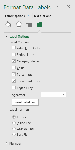
How to add data labels from different column in an Excel chart? This method will introduce a solution to add all data labels from a different column in an Excel chart at the same time. Please do as follows: 1. Right click the data series in the chart, and select Add Data Labels > Add Data Labels from the context menu to add data labels. 2. Pie Chart in Excel - Inserting, Formatting, Filters, Data Labels Click on the Instagram slice of the pie chart to select the instagram. Go to format tab. (optional step) In the Current Selection group, choose data series "hours". This will select all the slices of pie chart. Click on Format Selection Button. As a result, the Format Data Point pane opens. Prevent overlapping of data labels in pie chart - Stack Overflow However, the client insisted on a pie chart with data labels beside each slice (without legends as well) so I'm not sure what other solutions is there to "prevent overlap". Manually moving the labels wouldn't work as the values in the chart are dynamic. excel Share asked Apr 28, 2021 at 2:11 abc 359 3 17 You may be able to start with this answer Change the format of data labels in a chart To get there, after adding your data labels, select the data label to format, and then click Chart Elements > Data Labels > More Options. To go to the appropriate area, click one of the four icons ( Fill & Line, Effects, Size & Properties ( Layout & Properties in Outlook or Word), or Label Options) shown here.
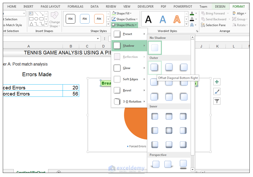
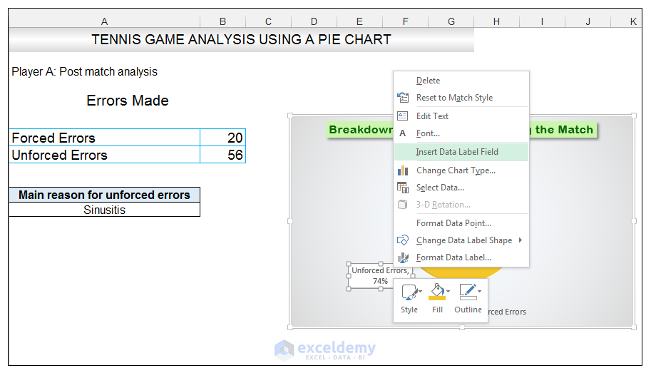
Add a DATA LABEL to ONE POINT on a chart in Excel All the data points will be highlighted. Click again on the single point that you want to add a data label to. Right-click and select ' Add data label '. This is the key step! Right-click again on the data point itself (not the label) and select ' Format data label '. You can now configure the label as required — select the content of ... How to Combine or Group Pie Charts in Microsoft Excel Click on the first chart and then hold the Ctrl key as you click on each of the other charts to select them all. Click Format > Group > Group. All pie charts are now combined as one figure. They will move and resize as one image. Choose Different Charts to View your Data Solved: Show multiple data lables on a chart - Power BI 09-07-2017 06:25 AM Is there a way to display multiple labels on a chart? For example, I'd like to include both the total and the percent on pie chart. Or instead of having a separate legend include the series name along with the % in a pie chart. I know they can be viewed as tool tips, but this is not sufficient for my needs. Creating Pie Chart and Adding/Formatting Data Labels (Excel) Creating Pie Chart and Adding/Formatting Data Labels (Excel)

Microsoft Excel Tutorials: Add Data Labels to a Pie Chart
Excel Pie Chart Multiple Labels Pie Charts in Excel - How to Make with Step by Step Examples. Excel. Details: Step 3: Right-click the pie chart and expand the "add data labels " option. Next, choose "add data labels " again, as shown in the following image. Step 4: The data labels are added to the …. › Verified 5 days ago.

How to: Setup a Pie Chart With No Overlapping Labels
How to display leader lines in pie chart in Excel? To display leader lines in pie chart, you just need to check an option then drag the labels out. 1. Click at the chart, and right click to select Format Data Labels from context menu. 2. In the popping Format Data Labels dialog/pane, check Show Leader Lines in the Label Options section. See screenshot: 3. Close the dialog, now you can see some ...

Microsoft Excel Tutorials: Add Data Labels to a Pie Chart
How to make a pie chart in Excel - Ablebits Adding data labels to Excel pie charts. In this pie chart example, we are going to add labels to all data points. To do this, click the Chart Elements button in the upper-right corner of your pie graph, and select the Data Labels option. Additionally, you may want to change the Excel pie chart labels location by clicking the arrow next to Data ...
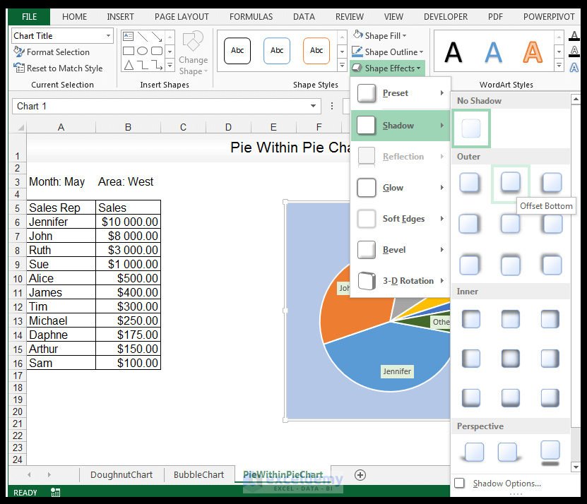
How to Create A Doughnut, Bubble and Pie of Pie Chart in Excel | ExcelDemy
Comparison Chart in Excel | Adding Multiple Series Under Same ... This window helps you modify the chart as it allows you to add the series (Y-Values) as well as Category labels (X-Axis) to configure the chart as per your need. Under Legend Entries ( S eries) inside the Select Data Source window, you need to select the sales values for the year 2018 and year 2019.

How to Make a Pie Chart in Excel & Add Rich Data Labels to The Chart!
How to Create Pie Charts in Excel (In Easy Steps) Select the range A1:D1, hold down CTRL and select the range A3:D3. 6. Create the pie chart (repeat steps 2-3). 7. Click the legend at the bottom and press Delete. 8. Select the pie chart. 9. Click the + button on the right side of the chart and click the check box next to Data Labels.
How to Make a Pie Chart in Excel & Add Rich Data Labels to The Chart!
How to Show Percentage in Pie Chart in Excel? - GeeksforGeeks Jun 29, 2021 · Select a 2-D pie chart from the drop-down. A pie chart will be built. Select -> Insert -> Doughnut or Pie Chart -> 2-D Pie. Initially, the pie chart will not have any data labels in it. To add data labels, select the chart and then click on the “+” button in the top right corner of the pie chart and check the Data Labels button.

Nested donut chart (also known as Multi-level doughnut chart, Multi-series doughnut chart ...
Formatting data labels and printing pie charts on Excel for Mac 2019 ... Here's a work around I found for printing pie charts. Still can't find a solution for formatting the data labels. 1. When printing a pie chart from Excel for mac 2019, MS instructions are to select the chart only, on the worksheet > file > print. Excel is supposed to print the chart only (not the data ) and automatically fit it onto one page.
How to Make a Pie Chart in Excel & Add Rich Data Labels to The Chart!
Multiple Data Labels on a Pie Chart - MrExcel Message Board So I have a table with 8 rows and 3 columns. This table includes: Column 1 - shipment name Column 2 - shipment cost Column 3 - shipment weight I have created a pie chart from this table, which covers the first two columns. Displayed next to each slice is a label with the shipment name, shipment cost, and percent share of the pie.

How to Make a Pie Chart in Excel
Create a multi-level category chart in Excel - ExtendOffice Create a multi-level category chart in Excel A multi-level category chart can display both the main category and subcategory labels at the same time. When you have values for items that belong to different categories and want to distinguish the values between categories visually, this chart can do you a favor.

Excel 3-D Pie Charts
Multiple data labels (in separate locations on chart) Re: Multiple data labels (in separate locations on chart) You can do it in a single chart. Create the chart so it has 2 columns of data. At first only the 1 column of data will be displayed. Move that series to the secondary axis. You can now apply different data labels to each series. Attached Files 819208.xlsx (13.8 KB, 264 views) Download
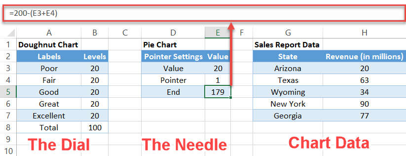
Excel Gauge Chart Template - Free Download - How to Create
Plot Multiple Data Sets on the Same Chart in Excel Jun 29, 2021 · You can further format the above chart by making it more interactive by changing the “Chart Styles”, adding suitable “Axis Titles”, “Chart Title”, “Data Labels”, changing the “Chart Type” etc. It can be done using the “+” button in the top right corner of the Excel chart.

r - Pie chart with multiple tags/info in ggplot2 - Stack Overflow
Excel Pie Chart Multiple Labels | Daily Catalog Add or remove data labels in a chart. Preview. 6 hours ago On the Design tab, in the Chart Layouts group, click Add Chart Element, choose Data Labels, and then click None.Click a data label one time to select all data labels in a data series or two times to select just one data label that you want to delete, and then press DELETE. Right-click a data label, and then click Delete.

Create a pie chart from distinct values in one column by grouping data in Excel - Super User
How to fix wrapped data labels in a pie chart - Sage Intelligence Right click on the data label and select Format Data Labels. 2. Select Text Options > Text Box > and un-select Wrap text in shape. 3. The data labels resize to fit all the text on one line. 4. Alternatively, by double-clicking a data label, the handles can be used to resize the label to wrap words as desired. This can be done on all data labels ...
Create a Pie Chart in Excel - Easy Excel Tutorial
How to Create a Pie Chart in Excel - Smartsheet Enter data into Excel with the desired numerical values at the end of the list. Create a Pie of Pie chart. Double-click the primary chart to open the Format Data Series window. Click Options and adjust the value for Second plot contains the last to match the number of categories you want in the "other" category.
How to Make a Pie Chart in Excel & Add Rich Data Labels to The Chart!
Pie Chart in Excel | How to Create Pie Chart - EDUCBA Pie Chart in Excel is used for showing the completion or main contribution of different segments out of 100%. It is like each value represents the portion of the Slice from the total complete Pie. For Example, we have 4 values A, B, C and D.
Automatically Group Smaller Slices in Pie Charts to one big Slice | Chandoo.org - Learn ...
How to create a chart in Excel from multiple sheets ... Nov 05, 2015 · Supposing you have a few worksheets with revenue data for different years and you want to make a chart based on those data to visualize the general trend. 1. Create a chart based on your first sheet. Open your first Excel worksheet, select the data you want to plot in the chart, go to the Insert tab > Charts group, and choose the chart type you ...
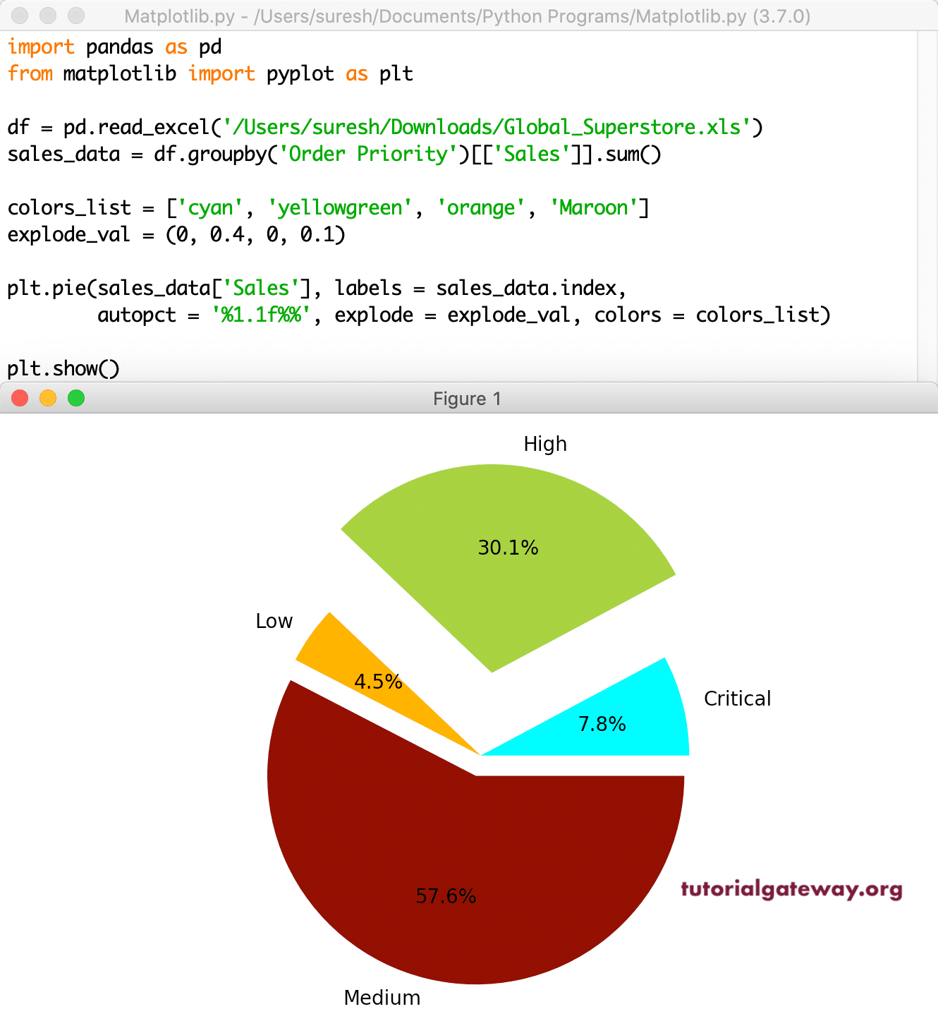
Python matplotlib Pie Chart
Add or remove data labels in a chart - support.microsoft.com Click the data series or chart. To label one data point, after clicking the series, click that data point. In the upper right corner, next to the chart, click Add Chart Element > Data Labels. To change the location, click the arrow, and choose an option. If you want to show your data label inside a text bubble shape, click Data Callout.
How to Make a Pie Chart in Excel & Add Rich Data Labels to The Chart!
Post a Comment for "43 multiple data labels excel pie chart"