44 excel column chart labels
Excel Custom Chart Labels - My Online Training Hub Note: Excel 2013 onward also requires this step if you have more than one series you want to position your labels above. Step 1: Select cells A26:D38 and insert a column Chart. Step 2: Select the Max series and plot it on the Secondary Axis: double click the Max series > Format Data Series > Secondary Axis: Step 3: Insert labels on the Max ... Create a multi-level category chart in Excel - ExtendOffice Select the dots, click the Chart Elements button, and then check the Data Labels box. 23. Right click the data labels and select Format Data Labels from the right-clicking menu. 24. In the Format Data Labels pane, please do as follows. 24.1) Check the Value From Cells box;
How to group (two-level) axis labels in a chart in Excel? Select the source data, and then click the Insert Column Chart (or Column) > Column on the Insert tab. Now the new created column chart has a two-level X axis, and in the X axis date labels are grouped by fruits. See below screen shot: Group (two-level) axis labels with Pivot Chart in Excel
Excel column chart labels
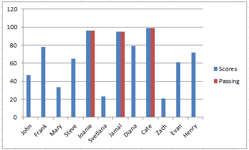
Excel charts: add title, customize chart axis, legend and ... Click anywhere within your Excel chart, then click the Chart Elements button and check the Axis Titles box. If you want to display the title only for one axis, either horizontal or vertical, click the arrow next to Axis Titles and clear one of the boxes: Click the axis title box on the chart, and type the text. How to Add Labels to Scatterplot Points in Excel - Statology Step 3: Add Labels to Points. Next, click anywhere on the chart until a green plus (+) sign appears in the top right corner. Then click Data Labels, then click More Options…. In the Format Data Labels window that appears on the right of the screen, uncheck the box next to Y Value and check the box next to Value From Cells. Text Labels on a Vertical Column Chart in Excel - Peltier Tech Right click on the new series, choose "Change Chart Type" ("Chart Type" in 2003), and select the clustered bar style. There are no Rating labels because there is no secondary vertical axis, so we have to add this axis by hand. On the Excel 2007 Chart Tools > Layout tab, click Axes, then Secondary Horizontal Axis, then Show Left to Right Axis.
Excel column chart labels. Dynamically Label Excel Chart Series Lines • My Online ... Select columns B:J and insert a line chart (do not include column A). To modify the axis so the Year and Month labels are nested; right-click the chart > Select Data > Edit the Horizontal (category) Axis Labels > change the 'Axis label range' to include column A. Step 2: Clever Formula How to I rotate data labels on a column chart so that they ... To change the text direction, first of all, please double click on the data label and make sure the data are selected (with a box surrounded like following image). Then on your right panel, the Format Data Labels panel should be opened. Go to Text Options > Text Box > Text direction > Rotate Custom Excel Chart Label Positions • My Online Training Hub When you plot multiple series in a chart the labels can end up overlapping other data. A solution to this is to use custom Excel chart label positions assigned to a ghost series.. For example, in the Actual vs Target chart below, only the Actual columns have labels and it doesn't matter whether they're aligned to the top or base of the column, they don't look great because many of them ... Change the format of data labels in a chart To get there, after adding your data labels, select the data label to format, and then click Chart Elements > Data Labels > More Options. To go to the appropriate area, click one of the four icons ( Fill & Line, Effects, Size & Properties ( Layout & Properties in Outlook or Word), or Label Options) shown here.
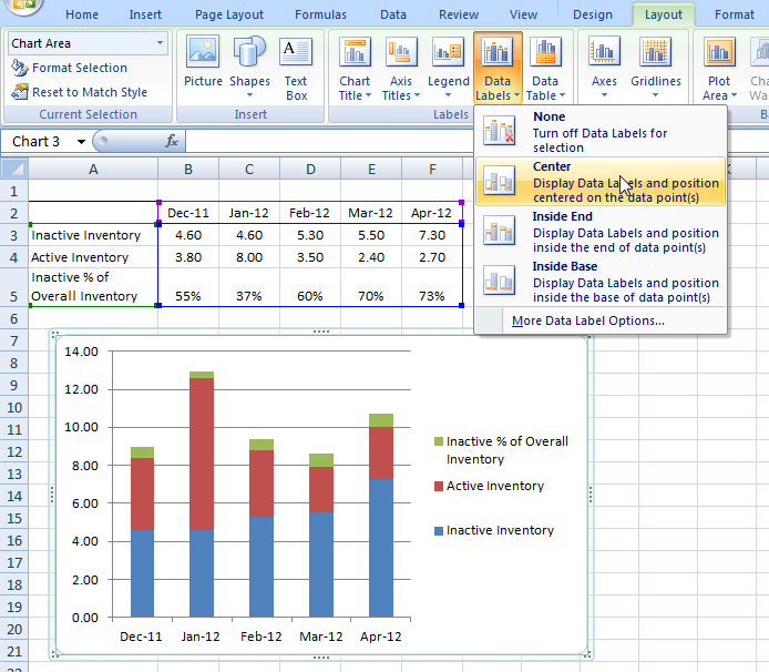
Add / Move Data Labels in Charts - Excel & Google Sheets ... Adding Data Labels Click on the graph Select + Sign in the top right of the graph Check Data Labels Change Position of Data Labels Click on the arrow next to Data Labels to change the position of where the labels are in relation to the bar chart Final Graph with Data Labels Excel tutorial: How to customize axis labels Instead you'll need to open up the Select Data window. Here you'll see the horizontal axis labels listed on the right. Click the edit button to access the label range. It's not obvious, but you can type arbitrary labels separated with commas in this field. So I can just enter A through F. When I click OK, the chart is updated. How to Create a Bar Chart With Labels Above Bars in Excel In the Format Data Labels pane, under Label Options selected, set the Label Position to Inside End. 16. Next, while the labels are still selected, click on Text Options, and then click on the Textbox icon. 17. Uncheck the Wrap text in shape option and set all the Margins to zero. The chart should look like this: 18. Chart Data Labels > Alignment > Label Position: Outsid ... Go to the Chart menu > Chart Type. Verify the sub-type. If it's stacked column (the option in the first row that is second from the left), this is why Outside End is not an option for label position. While still in the Chart Type dialog box, you can change the sub-type to clustered column (the option in the first row that is first on the left).
Change axis labels in a chart - support.microsoft.com Right-click the category labels you want to change, and click Select Data. In the Horizontal (Category) Axis Labels box, click Edit. In the Axis label range box, enter the labels you want to use, separated by commas. For example, type Quarter 1,Quarter 2,Quarter 3,Quarter 4. Change the format of text and numbers in labels Stagger long axis labels and make one label stand out in ... Stagger long axis labels and make one label stand out in an Excel column chart. The problem with long axis labels and the common solution. If you have long axis labels in a column chart, Excel will rotate them to fit the full labels in if the chart is not wide enough. How to Customize Your Excel Pivot Chart Data Labels - dummies If you want to label data markers with a category name, select the Category Name check box. To label the data markers with the underlying value, select the Value check box. In Excel 2007 and Excel 2010, the Data Labels command appears on the Layout tab. Also, the More Data Labels Options command displays a dialog box rather than a pane. Change axis labels in a chart in Office The chart uses text from your source data for axis labels. To change the label, you can change the text in the source data. If you don't want to change the text of the source data, you can create label text just for the chart you're working on. In addition to changing the text of labels, you can also change their appearance by adjusting formats.
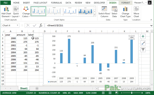
Custom Data Labels with Colors and Symbols in Excel Charts - [How To] - PakAccountants.com
How to Add Labels to Show Totals in Stacked Column Charts ... The chart should look like this: 8. In the chart, right-click the "Total" series and then, on the shortcut menu, select Add Data Labels. 9. Next, select the labels and then, in the Format Data Labels pane, under Label Options, set the Label Position to Above. 10. While the labels are still selected set their font to Bold. 11.

Labeling a Stacked Column Chart in Excel | PolicyViz
How to add data labels from different column in an Excel ... Right click the data series in the chart, and select Add Data Labels > Add Data Labels from the context menu to add data labels. 2. Click any data label to select all data labels, and then click the specified data label to select it only in the chart. 3.

34 How To Label Excel Columns - Labels For You
How to Insert Axis Labels In An Excel Chart | Excelchat Figure 2 - Adding Excel axis labels. Next, we will click on the chart to turn on the Chart Design tab. We will go to Chart Design and select Add Chart Element. Figure 3 - How to label axes in Excel. In the drop-down menu, we will click on Axis Titles, and subsequently, select Primary Horizontal. Figure 4 - How to add excel horizontal axis ...

Labeling a Stacked Column Chart in Excel | PolicyViz
Add or remove data labels in a chart Click the data series or chart. To label one data point, after clicking the series, click that data point. In the upper right corner, next to the chart, click Add Chart Element > Data Labels. To change the location, click the arrow, and choose an option. If you want to show your data label inside a text bubble shape, click Data Callout.
31 How To Label Excel Columns
How to Use Cell Values for Excel Chart Labels Select the chart, choose the "Chart Elements" option, click the "Data Labels" arrow, and then "More Options." Uncheck the "Value" box and check the "Value From Cells" box. Select cells C2:C6 to use for the data label range and then click the "OK" button. The values from these cells are now used for the chart data labels.
Clustered/Stacked Filled Bar Graph Generator
Edit titles or data labels in a chart - support.microsoft.com On a chart, click the label that you want to link to a corresponding worksheet cell. On the worksheet, click in the formula bar, and then type an equal sign (=). Select the worksheet cell that contains the data or text that you want to display in your chart. You can also type the reference to the worksheet cell in the formula bar.

Changing Axis Labels in PowerPoint 2013 | PowerPoint Tutorials
How to Make a Column Chart in Excel: A Guide to Doing it Right Excel offers a 100% stacked column chart. In this chart, each column is the same height making it easier to see the contributions. Using the same range of cells, click Insert > Insert Column or Bar Chart and then 100% Stacked Column. The inserted chart is shown below. A 100% stacked column chart is like having multiple pie charts in a single chart.
31 How To Label Excel Columns - Labels For Your Ideas
How to add total labels to stacked column chart in Excel? Select the source data, and click Insert > Insert Column or Bar Chart > Stacked Column. 2. Select the stacked column chart, and click Kutools > Charts > Chart Tools > Add Sum Labels to Chart. Then all total labels are added to every data point in the stacked column chart immediately. Create a stacked column chart with total labels in Excel
Excel Dashboard Templates How-to Put Percentage Labels on Top of a Stacked Column Chart - Excel ...
Adding Labels to Column Charts | Online Excel Training ... We'll need to change the chart type to the clustered column chart. So I'll escape, right-click, change chart type, and select the clustered column chart. Now I'll select my data labels, right-click, and format data labels, and here we have an option for outside end under position. I'll select it and then click close.
Change Chart Style in Excel | How to Change the Chart Style in Excel?
How to create Custom Data Labels in Excel Charts Create the chart as usual. Add default data labels. Click on each unwanted label (using slow double click) and delete it. Select each item where you want the custom label one at a time. Press F2 to move focus to the Formula editing box. Type the equal to sign. Now click on the cell which contains the appropriate label.
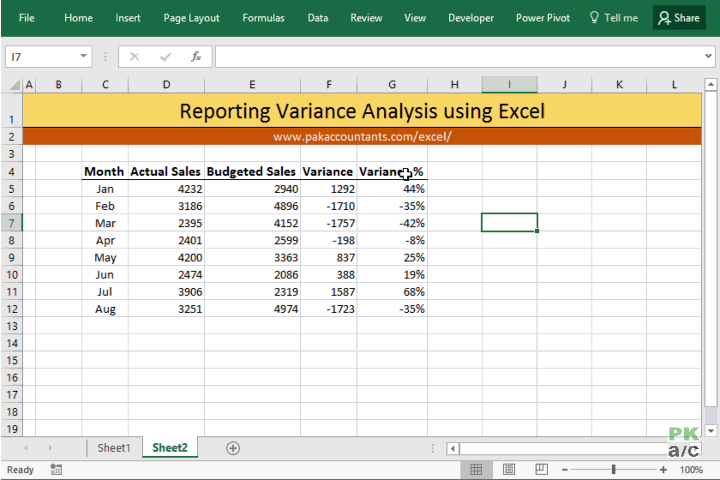
10 ways to present variance analysis reports in Excel - PakAccountants.com
Text Labels on a Vertical Column Chart in Excel - Peltier Tech Right click on the new series, choose "Change Chart Type" ("Chart Type" in 2003), and select the clustered bar style. There are no Rating labels because there is no secondary vertical axis, so we have to add this axis by hand. On the Excel 2007 Chart Tools > Layout tab, click Axes, then Secondary Horizontal Axis, then Show Left to Right Axis.

Create a column chart with percentage change in Excel
How to Add Labels to Scatterplot Points in Excel - Statology Step 3: Add Labels to Points. Next, click anywhere on the chart until a green plus (+) sign appears in the top right corner. Then click Data Labels, then click More Options…. In the Format Data Labels window that appears on the right of the screen, uncheck the box next to Y Value and check the box next to Value From Cells.
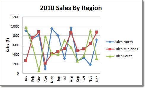
Excel - Line Chart
Excel charts: add title, customize chart axis, legend and ... Click anywhere within your Excel chart, then click the Chart Elements button and check the Axis Titles box. If you want to display the title only for one axis, either horizontal or vertical, click the arrow next to Axis Titles and clear one of the boxes: Click the axis title box on the chart, and type the text.

How to add total labels to stacked column chart in Excel?
Text Labels on a Vertical Column Chart in Excel - Peltier Tech Blog
How-to Put Percentage Labels on Top of a Stacked Column Chart - Excel Dashboard Templates
Post a Comment for "44 excel column chart labels"